Digital pulse processors. Theory of operation

Digital pulse processors are widely used in nuclear instrumentation and are the basis of most systems sold by Amptek. A digital pulse processor performs the same functions as an analog amplifier/driver, but has effective performance advantages that have led to its widespread adoption in applications where the lowest noise and highest count rates are simultaneously required. Although the functions of a digital pulse processor are the same as those of an analog driver, the implementation is different and some of the concepts and terminology are different. The purpose of this application note is to compare the analog and digital driver, to help users understand the digital processors, and to explain their advantages and disadvantages.

Simplified diagrams

Figures 1 and 2 show simplified schematics of an analog and digital amplifier-shaper , respectively . Both have the same detector and charge-sensitive preamplifier circuits. In both cases, the preamplifier produces an output signal that consists of small pulses (steps) with an amplitude of millivolts. In both cases, the preamplifier pulses are differentiated so that the voltage step can be measured. An integrator (also called a low-pass filter) improves the signal-to-noise ratio. In both cases, the output pulses are digitized, and histograms of the pulse amplitudes are stored in memory. These key elements are the same in both systems.

Figure 1. Schematic diagram of a simple analog pulse shaper (with CR-RC2 shaper)

Figure 2. Simplified diagram of an “ideal” digital pulse processor

Before moving on to a more detailed study of the operation of a digital pulse processor, it is necessary to become familiar with the basic terms used in nuclear electronics; Figure 3 shows an illustration of a unipolar pulse.

Figure 3. Illustration of a typical unipolar pulse shape

Pulse duration is the time during which the pulse amplitude is not zero. Because of the difficulty of defining the exact value of "zero" amplitude, it is usually defined as the FWHM (full width at half maximum), the time during which the pulse amplitude is greater than or equal to half the peak height.

Peak Height - The height of the pulse measured from the peak to the baseline. Peak Time - The time required to shape the pulse from the baseline to the peak, related to the time constant of the shaper amplifier.

Baseline - the voltage value in the absence of a pulse from a detected event. In nuclear electronics, the pulse height is measured relative to the baseline, which does not necessarily have to be zero.

Base-line stabilizer (BLS) its task is to fix the reference point of the pulse amplitude regardless of temperature and time drifts of electronic components and effects of high counting rate (dynamic shifts on separating capacitors and micro-heating of the input stages of operational amplifiers).

Let us now consider the functional diagram of the pulse shaper. The analog system shown in Fig. 1 is inferior to the pulse shaper shown in Fig. 5 (left). The differentiator is an RC high-pass filter. The front passes through the preamplifier, and then the voltage exponentially decays back to the original (baseline) with a time constant T _diff . The integrator is a low-pass filter with a response time of T _int . There are many types of amplifier-shapers (semi-Gaussian, pseudo-Gaussian, quasi-triangular, etc.), which use different low-pass filters, the pulse shapes from different amplifier-shapers are shown in Figure 4.

Figure 4. Illustration of pulse shapes obtained from different amplifiers-shapers. Each of them has a constant shaping time constant of 1 µs, but the integrators - low-pass filters, use different transfer functions

General properties:

RC-CR: Very simple to implement, but generally has poor performance, i.e. noise, dead time, and stability.

• Bipolar: Pulse drawdown allows for good baseline stability, is easy to implement, but has a long pulse duration and, as a consequence, a large dead time value and poor noise characteristics
• Semi-Gaussian and Pseudo-Gaussian: Implemented using active filters (complex pole pairs). When used with active baseline generation, they provide good performance using analog components.
• Quasi-Triangular: Also implemented using active filters in analog components. This is very close to the "ideal" transfer function, for optimum performance, but is relatively complex.
• Trapezoidal: Implemented using digital processing. Also very close to ideal, has a finite impulse response and increased performance at high count rates.

More sophisticated shaping amplifiers using a mixed complex pole pair have a fast return to the baseline with a more symmetrical shape. Typically the pulse shape is approximated by a Gaussian with a shaping time characteristic t. The peak time is approximately 2.2t, with a comparable duration of half the maximum voltage, but the tail persists for a longer time. A baseline generator (BLR) produces a baseline from which each peak is measured. Without a BLR, the ac current from the differentiator would drop at high count rates, since the dc output must be zero. The analog peak is detected and the circuit captures the peak amplitude, which is then digitized. This single digital sample represents a pulse, so the ADC must be linear, but not necessarily very fast, since it only digitizes one sample of the pulse.

In the “ideal” digital system shown in Fig. 2, the preamplifier signal is digitized directly using a fast ADC. This is a differential use of a discrete differentiating circuit. The signal is sent to a low-pass filter, which integrates the differentiator output. The two blocks labeled “process” represent the algorithms that are applied to the input signals and that distinguish one digital processor from another. The most common low-pass filter produces a triangular waveform at the output. Trapezoidal pulses are also easily synthesized, as are more complex shapes such as a “spike.” The values are already digitized, so the detected digital peak is sent to a histogram memory. The histogram memory works as in a traditional multichannel amplitude analyzer. When a pulse with a particular peak value occurs, the counter in the corresponding memory cell is incremented. The result is an array containing, in each cell, the number of events with the corresponding pulse value. This energy spectrum is the main output of the processor. The integrator output can also be fed to a DAC, so the user can view the pulses on an oscilloscope, but the system does not have to generate an analog pulse waveform. The pulse shaper is shown in Fig. 5 (right).

Fig. 5 Left: Pulse shapes in an analog pulse shaper. They correspond to a quasi-triangular shaper using complex poles that are closest to a triangle. Right: Pulse shapes in a digital pulse processor with triangular and trapezoidal shapes.

Real digital processor

A real digital processor has several key differences from the "ideal" one. Moreover, due to the dynamic range, it is not practical to directly digitize the preamplifier output. Each preamplifier output has a step, millivolt in amplitude, that moves along a baseline that can be several volts and change over time. The step must be digitized at 10 to 14 bits, and there is simply no ADC that combines the precision of the preamplifier output dynamic range with the necessary speed. Therefore, the preamplifier output is passed to an analog pre-filter, which allows the step to be accurately digitized. Several different approaches are used to remove the baseline and amplify the step before digitization. In addition, there are various implementations of the differentiator, from the low-pass filter or integrator, and the peak detection logic.

Conclusion: Advantages and Disadvantages of Digital Filtering

The digital processor has several key advantages , listed here and explained below. The digital pulse processor has better performance (low noise and high count rate at the same time), greater flexibility for customization to the specific application, better stability and reproducibility.

• Researchers have long sought ideal filters for use in nuclear electronics that give the best signal-to-noise ratio at a given count rate. The ideal transfer function cannot be easily produced in a practical operational amplifier circuit, but a digital processor comes closest to the ideal.
• There is no dead time associated with signal detection and digitization, so the digital processor has a higher throughput than an analog system. In addition, because it has a finite impulse response, aliasing and other pulse overlap effects are reduced. The performance advantage of the digital processor is especially noticeable at high count rates.
• In an analog pulse processor, most of the parameters are determined by resistors and capacitors. It is impractical to have many different configuration parameters in an analog system. In a digital system, it is possible to have many more shaping time constants, BLR parameters, etc., so that the user can easily adapt the system to the needs of the task, improving the operating efficiency.
• Since an analog system is built on resistors and capacitors, its stability is limited by the constancy of these components, and its reproducibility by their errors. In a digital system, stability and reproducibility are much better because they are set from several very accurate sources, such as a quartz oscillator for setting the time.

There are disadvantages to the digital processor. First, it tends to dissipate more power: an ADC with suitable speed and accuracy dissipates more power than many analog designs. Second, the design is more complex than an analog amplifier-shaper.

Advantages of digital filtering

Finite impulse response:

In an analog shaper, an incoming pulse produces an exponential tail from the differentiator, which takes an infinite amount of time to return to zero. This is called an "infinite impulse response" or IIR. The output is negligible after a finite time, but it is nonzero for a long time, typically many times the nominal "width" of the pulse. Subsequent pulses "sit" on the tail of earlier pulses. Since the high-pass filter output is DC, the baseline shifts at the count rate: over a large span, the average pulse value is important and depends on the duration, but has a small tail amplitude. Therefore, aliasing occurs, and the baseline shifts the IIR output of the analog differentiator. Aliasing is an event in which two or more pulses overlap in time (Figure 6).

Figure 6. Illustration of pulse superposition

This plot shows five incidents that occur at random time intervals, since nuclear decay is a random process. The individual pulses are highlighted by the black lines, while the blue dots represent the sum of the overlapping pulses that was measured. The first pulse, on the left, is isolated in time and its amplitude is measured at the correct height. The next two partially overlap, with a saddle between the peaks. Two pulses will be recorded, and the first will have the correct pulse height, but the amplitude of the second pulse will be measured incorrectly. An overlap of two pulses where there is no saddle between the peaks appears as a single pulse (they are not resolvable) with the wrong height. If the two overlaps occur close enough in time, the resulting amplitude is the sum of the individual pulses.

In a digital shaper, the response to a pulse is a rectangular differentiator response: the response goes to zero after k pulses. It has a "finite impulse response" (FIR), meaning that any input has zero effect after a finite amount of time. This is the main difference from an analog shaper. Whatever happens at the input of the DPP results in a zero at the output after a certain period of time. This greatly improves the efficiency of the DPP at high count rates, reduces aliasing and baseline shift, etc.

Flat Top Restoration

In an analog shaper, the preamplifier provides a fast rise and flat top of the signal being processed. The differentiator passes the pulse, but then immediately begins to decay. If the front rises slowly, its shaping time decreases exponentially and the pulses do not reach full amplitude, as shown in Figure 7 (left). Every X-ray detector has a charge collection time, but the pulse shaping time is long enough that the charge collection time can be ignored. In a planar detector, such as the Amptek 6 mm2 ^silicon detector, it takes 0.1 (0.3) ms for electrons (holes) to cross 500 mm of depletion region. Depending on the X-ray penetration depth, the duration of the current produced in the preamplifier is from 0.1 to 0.3 ms. If a pulse shape with T _flat < 0.3 ms is used, only a fraction of the charges will be measured. The loss of pulse height with rise time is called ballistic deficit and affects resolution when rise time varies from one pulse to the next.

Figure 7. Schematic diagram of the output differentiator for the analog (left) and digital (right) shaper

In this example, the peak time is 4.8 µm sec, 500 ns rise time leads to a 0.5% loss of pulse height. The problem occurs because the analog "differentiator" does not receive the actual derivative function and therefore does not form a flat top. The advantage of the digital differentiator is that it actually implements differentiation of the digital derivatives, so a real flat top is obtained, as can be seen in Fig. 7 (right). The front and flat top have the same shape as the pulse preamplifier. Therefore, the digital processor is protected from ballistic deficit and has a flat top duration several times shorter.

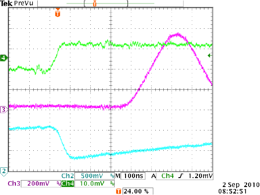
In the silicon drift detector (SDD), there are also differences in the charge collection time. The physical mechanism is different from the planar detector and the rise time depends on the details of the electrode structure, the voltage is offset, but all SSDs show different charge collection times. Figure 8 shows the waveforms obtained with the Amptek SSD. The green waveform shows the preamplifier, with a rise time of 40 to 200 ns (the slow-rising pulses occur near the outer edge of the electrically active region).

Figure 8. Oscilloscope traces illustrating the pulse rise time measurement. The green trace shows the preamplifier output, the blue trace shows the ADC input, and the pink trace shows the slow channel for 100 ns peak and 50 ns flat top times.

The spectra with the ballistic deficit effect are shown in Figure 9. These plots were obtained using a 55Fe source at low count and without external collimation. The plot on the left corresponds to T _peak = 0.1 ms and T _flat from 0.025 to 0.2 ms. A longer T _flat leads to a narrower peak. The plot on the right corresponds to T _peak = 0.4 ms and the same range of T _flat . In the case of a larger T _peak , even a short T _flat time leads to a decrease in the ballistic deficit.

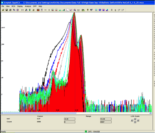
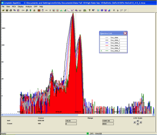
Figure 9. Spectra corresponding to Tpeak = 100 ns (left) and 400 ns (right) with DP5 25mm2 Amptek SDD

What can be done about the ballistic deficit?

• Increase T _peak and T _flat . This will improve resolution but will reduce the maximum count rate. For T _peak > 2 ms, Amptek recommends T _flat > 0.2 ms because it does not have a big impact on throughput.

• Increase the bias voltage. This will reduce the rise time by half;

• An external collimator must be used. If the flow is high enough, it is better to use the Amptek mini-X;

• In principle, one can use the thermal resistance of the detector to cut off slow events. This method is called electron collimation because it effectively reduces the active area;

• Use software to handle ballistic deficits on the spectrum.

Overlay

R

Figure 10 shows the output pulse waveforms from three different pulse shapers, all adjusted to give the same pulse width as measured at full width at half maximum. The red trace shows the output of the simplest shaper, an analog RC-CR. The blue trace shows the waveform from a high-end analog shaper, a quasi-triangular shaping amplifier, using 6 poles of low-pass filtering (three complex pole pairs). The black trace is from a digital trapezoid shaper. The most important thing to note is that although they have the same pulse width at FWHM, the digital shaper will show no overlap if the two pulses are separated by more than (t _peak + t _flat ). The two analog shapers have exponential tails that are many times the FWHM. Pulses that overlap during this time will overlap.

Figure 10. Graph showing pulses generated in three different pulse shapers. All have essentially the same pulse width, which is specified by the FWHM.

There are two advantages of digital shaper. First, digital shaper has less aliasing (even with the same FWHM). Second, digital system has clear aliasing time: due to the symmetry of the pulse, there is no aliasing after a fixed time. Analog shapers must use alias rejection of an interval much longer than the peak time. The bandwidth, i.e. dead time, is reduced due to pulse shaping, which is longer in the analog system. Therefore, compared with analog shapers, digital system has less aliasing and high bandwidth.

There are several issues with pileup rejection (PUR). First, PUR only functions if T _fast < T _peak . Second, if T _fast is slightly less than T _peak , no pileup rejection will occur. For example, with T peak = 100 ns and T flat = 12 ns, the actual dead time is ~ 140 ns. With T _fast = 50 ns, the resolution between a pair of pulses in the fast channel is ~ 100 ns. In this case, PUR only rejects pulses lagging between 100 and 140 ns. Third, if T _flat < T _fast , the "sum peak" will not actually be a peak, but will have a rather complex shape. Figure 11 illustrates this case.

Figure 11. The spectrum shows the duration of the flat top when rejecting the pulse histogram overlaps.

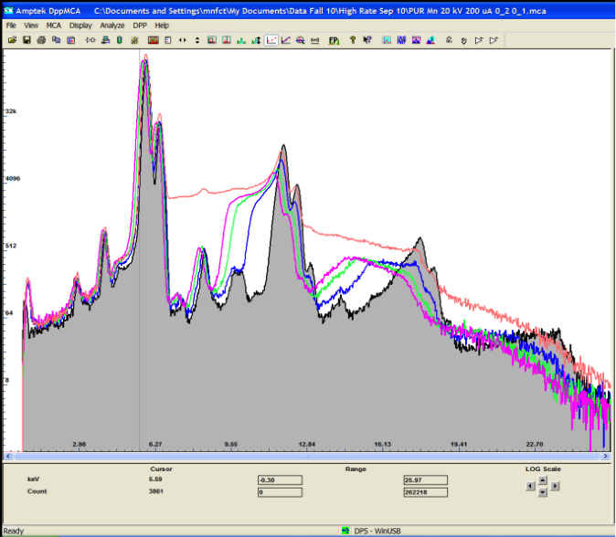
The values were obtained with T _peak = 0.4 ms. The orange spectrum is obtained with alias rejection disabled. The gray filled spectrum shows PUR enabled for T flat = 0.2 ms. The other spectra are obtained with shorter T _flat values . The ballistic deficit problem is best addressed with T _flat > 100 ns, this also helps reduce artifact accumulation when alias rejection is enabled. Amptek recommends using T _flat > 100 ns, and T _flat > 200 ns for T _peak > 2 ms or so to help reduce these effects. The blue spectrum is for T _flat = 75 ns. When the flat duration is shorter than the alias rejection interval, pulses may overlap each other, but they do not result in a combined peak. The green and red spectrum are for T _flat = 25 and 50 ns. Spectrum analysis software is typically designed to correctly remove aliased peaks. To get a good overall peak, you need to extend the flat top, which of course reduces throughput.

On the oscillogram (Fig. 12), the pulse shape is equal to the sum of two trapezoids shifted in time. If two events are separated by more than the duration of the flat top, then the amplitude of the peak depends linearly on the delay between the events. If the delay is less than the duration of the flat top, then the sum of the peak values is obtained on the graph.

Figure 12. Oscillograms showing pulse overlaps. Pink trace is the ADC input. Light blue trace is the generated output (peak time 2.4 ms). Blue trace is the "ICR" signal indicating that the pulse was detected in the fast channel.

Signal to noise ratio

The main task of the spectrometric amplifier is to linearly transmit the amplitude values of signals coming from radiation detectors. In this case, it is allowed to change the shape of the signals. This means that the filtering circuits of the amplifier can be made such that the main spectrum of signals passes through them, and the noise spectrum is limited as much as possible. In this case, we get the optimal signal-to-noise ratio. The signal at the output of the optimal filter has the shape of two intersecting curves. Such a filter provides the best signal-to-noise ratio. Real filters, as a rule, have other characteristics, and their signal-to-noise ratio is worse. It is convenient to compare filters using the noise excess ratio K _n.sh = ƞ∞/ ƞ, showing how many times ƞ∞ of the optimal filter exceeds ƞ of a given system. The main indicators of different types of pulses are given in Table 1. Here K _n.sh. are calculated under the condition that the intensity of serial and parallel noise is the same, and the amplitude of the output signal is normalized to unity.

Table 1. Noise excess factors and pulse shapes of some shaping circuits

Researchers have long concluded that for a fixed pulse duration, when serial noise is dominant, the optimum signal-to-noise ratio is provided by a pulse in the form of a regular triangle, and in the form of a “spike” when parallel noise is dominant. Serial noise is the electronic noise that arises from the components used with the detector. As a rule, the noise corresponds to the voltage in the preamplifier and arises primarily from noise in the input channel of the preamplifier. Parallel noise is the electronic noise that arises from components connected in parallel with the detector. As a rule, it arises mainly from thermal noise in the detector and parallel resistances.

Analog shapers approximate the triangle, but a digital processor has a transfer function much closer to this ideal. The equivalent noise floor for a radiation detection system is characterized by the noise indices for the serial and parallel noise generators, As and Ap, for a given peak time t _peak . The noise can be written:

where L _leak is the leakage current through the detector, R _p is the parallel resistance with the detector, C _in is the total input capacitance, g _m is the admittance of the field-effect transistor and e _peak is the 1/f noise. The key point is the noise indices Ap and As depending on the details of the driver amplifier.

The table below shows the noise indices and FWHM pulse widths for three common conditioning amplifiers similar to those shown in Figure 9. If the peak time is constant, the trapezoidal and Gaussian have the same parallel noise index, but the digital has a lower serial noise index and the Gaussian has a longer duration, leading to more aliasing. One must be careful in this comparison, since the peak time is not really the key parameter. In Figure 9, all the pulses have the same peak time but different durations. The longer the pulse widths, the more aliasing will occur, even with the same peak time. There is also the problem of finding an optimal filter that allows one to calculate the baseline offset with minimal noise error in a finite time interval before the spectrometric pulse appears, store it, and subtract it from the superposition of signal, noise, and DC offset. The key point is that the digital pulse processor with its true trapezoid has low noise indices and a narrower time-domain width than comparable analog shapers. Therefore, it simultaneously reduces electronic noise and aliasing.

Table 2. Noise indices and pulse width (FWHM) for three common shaper amplifiers

Multi-channel pulse amplitude analyzer (MCA). Bandwidth

There are two sources of dead time in an analog system: some pulses may be lost (not detected) because (a) the pulses overlap in time, or (b) the peak is detected but the digital converter is busy. Most multichannel amplitude analyzers use ADCs that are only microseconds long, but even if the analog pulses do not overlap in time, the count will be lost due to the digital converter's dead time. In a digital processor, there is no dead time associated with sampling the peak. The entire pulse waveform has already been digitized at a high speed, say 20 MHz. There will be a few clock cycles needed to update the histogram memory, but this is negligible. Therefore, a digital system does not have dead time associated with sampling the peak. It has dead time associated with the pulse width, as discussed above.

Linearity

In an analog system, the nonlinearity of the ADC has a large impact on the nonlinearity of the system. Since a multi-channel pulse amplitude analyzer makes a single peak height measurement, any nonlinearity in the size of the ADC steps will result in nonlinear pulse height measurements. One common ADC approach to smoothing out the nonlinearity is to add random numbers to the pulse, digitize it, and then subtract the random numbers. The result is several ADC codes that are used to measure the voltage of a single pulse height. In a digital system, each pulse height is the sum of many different ADC measurements, essentially using many different ADC codes. This gives the digital system much improved linearity.

Configurability.

In an analog pulse processor, most of the parameters are determined by resistors and capacitors. In a pseudo-Gaussian shaper, for example, the shaping time is determined by a set of fourteen resistors and capacitors. An analog amplifier shaper with four shaping time constants would require four different sets of all these components. It is impractical to have many different configuration parameters in an analog system.

In a digital system, the shaping time is set to the number of digital delay cycles and in the accumulator. It is easy to switch between the time shaper and the 20 MHz clock, the step size of 50 ns, giving very fine adjustment. Such processing options are not possible in an analog circuit. For example, some digital processors adjust the peak time on a pulse-by-pulse basis: if the interval between two pulses is small, then a short peak time is used, adding a little noise, but eliminating aliasing and count loss. In a digital system, many more parameters and configuration options can be easily obtained. These parameters include not only the shaping time, but also the baseline recovery parameters, alias rejection parameters, etc. The digital system has many more configuration parameters, so the user can easily adapt the system to the needs of the problem at hand, increasing the efficiency of the work.

Stability and reliability.

Since the analog system is based on resistors and capacitors, its stability is limited by the stability of these components and the reproducibility of their errors. The temperature coefficient of resistors and capacitors causes the growth and formation of a temperature gradient. Errors among resistors and capacitors cause differences between nominally identical pulse shapes when moving from one configuration to another. The gain accuracy is usually set with a potentiometer and is difficult to return to a previous setting, and it is also difficult to fine-tune two systems to match each other.

In a digital system, stability and repeatability depend on a few very precise sources, such as a quartz oscillator to set the time. In this case. Temperature drift is much lower. Repeatability is much better. In a digital system, where the gain is set digitally, you can return to the previous parameters exactly. In addition, the failure rate in FPGAs is very low compared to the failure rate of many discrete components, with their soldered connections.

Conclusion

The digital processor has inherent performance advantages over the analog shaper. It has a finite impulse response, reduced aliasing and baseline shift, it provides better noise filtering (for the same pulse width), it reduces ballistic deficit and improves linearity, it has better configurability, stability, and reliability.

Its main disadvantage is that a fast ADC consumes significantly more power than the operational amplifier and the slow ADC used in the analog driver. When the best performance, lowest noise, and highest count rate operations are required, a digital processor is the best solution.